Genome-wide association studies
Introduction
A genome-wide association study (GWAS) is a hypothesis-free method of finding genetic factors that are associated with a trait or disease. Any two individuals randomly sampled from the population will differ in only about 0.5% of their genetic makeup:
0.1%: Single nucleotide polymorphisms (SNPs)
0.4%: Structural variations including copy number variations (CNVs) and large scale insertions, deletions, or inversions
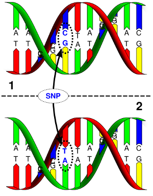
A SNP occurs when a single base of DNA is substituted with another, resulting in a polymorphism (for example, a C–G basepair being subtituted with a T-A basepair). SNPs occur once in every 100–1000 basepairs (BP) on average. Currently there are about 80 million known SNPs in the human genome.
GWAS typically analyse common SNPs (with frequencies >= 1%). In a GWAS, every SNP available in the data set is tested, so there will be as many tests as their are SNPs. A typical dataset will contain hundreds of thousands to several million SNPs.
Performing an association test
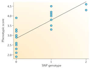
An association test is performed by comparing a genotype at a particular SNP marker to a phenotype (a trait or disease). This test is usually done within a regression framework, using linear regression for continuous/quantitative phenotypes (like height) or a logistic regression for a binary or case/control phenotype (like disease status).
At each SNP there are typically two alleles, for example C and T. This allows for four possible genotypes: CC homozygote, CT or TC heterozyogotes, and TT homozygotes. The basic association tests assumes that substituting one allele for the other has an additive effect on the phenotype. This means that the model assumes that the average difference in phenotype between the CC genotype and the CT genotype is the same as between the CT and TT genotype.
To run the regression, the SNP genotype is encoded to a number as a count of one of the alleles (which allele is chosen is arbitrary, but traditionally it is the minor allele). The chosen allele is called the “effect allele”. In this example, if the T allele is chosen as the effect allele, then the numeric encoding is the number of T alleles in the genotype: CC = 0, CT and TC = 1, and TT = 2. This numeric representation can then be entered into a regression formula:
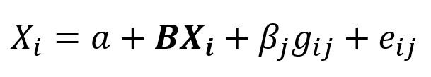
where Yi is the phenotype of participant i, Xi is a vector of covariates for participant i, gij is the numerical genotype for participant i at SNP j, and eij is the error term. B is a vector of regression coefficients for the covariates and βj is the regression coefficient for SNP j. From the fitted regression model, the beta coefficient βj for the SNP represents the average substitution effect of having one additional copy of the effect allele.
Binary traits like disease status are analysed as case-control studies using logistic regression. In a case-control analysis, the beta coefficient represents the change in log-odds of having the disease for every additional copy of the effect allele. Exponentiating the beta coefficient,  , converts the effect size to an odds ratio.
Population stratification
One possible confounder when performing association tests is that many allele frequencies differ between populations and subpopulations, while disease prevalences also differ. This can create false associations between SNPs and diseases.
These systematic differences in allele frequencies between subpopulations is called “population stratification”. The most obvious cause of stratification is ancestry but it can also be caused by confounding between environmental factors and geography. A principal components analysis of genetic variation across the whole genome can be used to visualise this variation.
A statistical summary of the first two major dimensions of variation (PC = principal component). Each participant is plotted at their genetic coordinates using text label for their country of origin. The plot resembles the geographic relationship between each country.
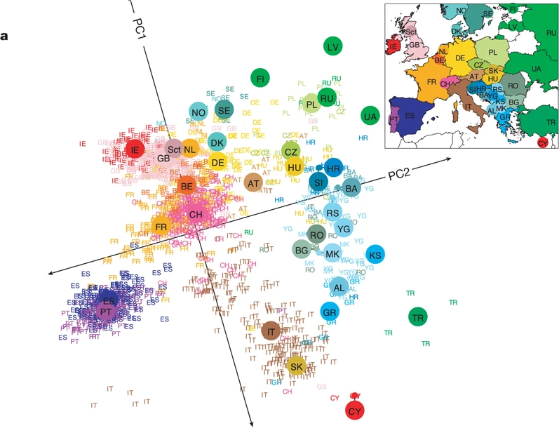
Novembre et al “Genes mirror geography within Europe” 2008
The association between polygenic burden for traits and diseases and UK geography can be explored on the Genes & Geography in Great Britain web app, based on the paper Abdellaoui et al. “Genetic correlates of social stratification in Great Britain” 2019.
There are other sources of false positives, such as technical artifacts and batch effects when cases and controls are genotyped separately, but these are usually easier to detect and remove during standard quality control (QC) processing.
Multiple testing and significance
Genetic data can contain hundreds of thousands or millions of variants. What p-value should be used to determine statistical significance?
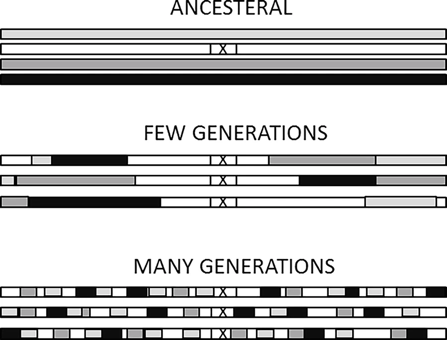
Standard methods to correct for multiple testing, such as Bonferroni correction based on the number of tests, are too conservative. This is because SNP markers are not independent. Instead, SNPs that are physically close to each other on a chromosome tend to be correlated (termed “linkage disequilibrium”). This correlation is because recombination breaks up the linkage between a mutation and the rest of the chromosome as it is passed down through generations.
Hettiarachchi, G., Komar, A.A. (2022). GWAS to Identify SNPs Associated with Common Diseases and Individual Risk: Genome Wide Association Studies (GWAS) to Identify SNPs Associated with Common Diseases and Individual Risk. https://doi.org/10.1007/978-3-031-05616-1_4
The p-value threshold can be derived empirically from the number of independent genomic regions, which has been determined to be about 1 million. Thus a multiple testing correction of p <= 0.05/1,000,000 = 5 × 10⁻⁸ is used as the standard significance threshold in GWAS.
The lack of independence among SNPs also means that, for any genomic region found to be associated with the trait, it is necessary to select one or more SNPs that represent or cause the signal in that region (“clumping”).
Summarising the results
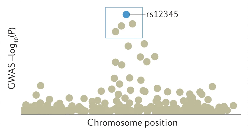
The results from a genome-wide association study can be visualised using a graph that is called a Manhattan plot. The plot features results for each SNP plotted by chromosome and basepair position on the x-axis versus transformed p-values on the y-axis. The p-values are transformed as the negative log 10 [-log10(P)], which turns very small p-values into large, positive numbers.
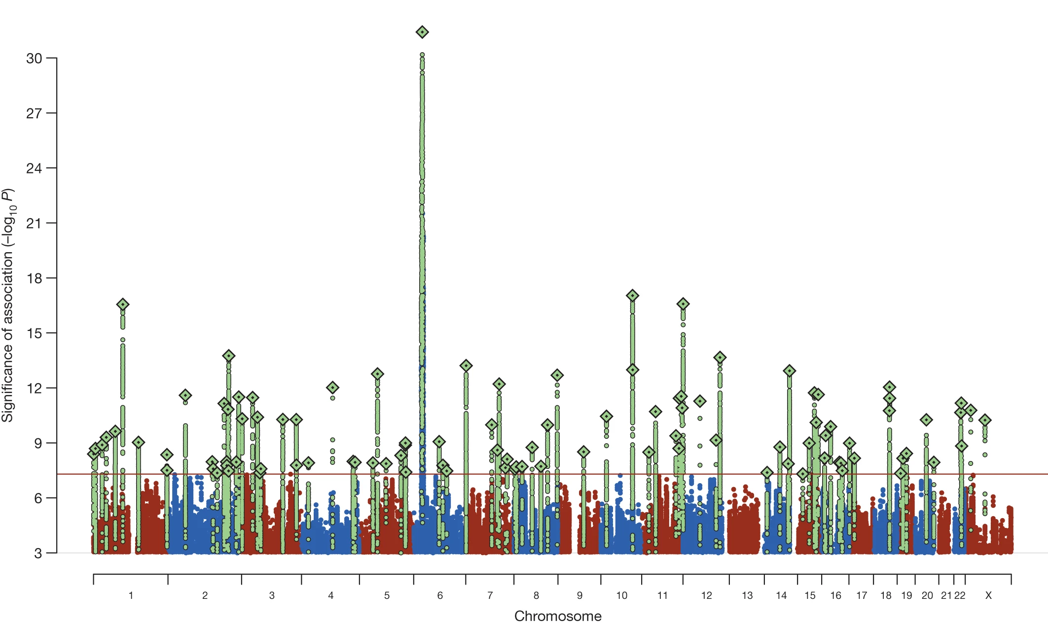
To summarise the results, SNPs that nearby and in linkage disequilibrium with each other are clumped together, and the SNP within the clumped region with the smallest p-value is selected. There are other more advanced techniques for determining the causal SNP or set of SNPs in a region, such as conditional-and-joint analysis and finemapping.

Once the SNPs are selected, the GWAS signals can be integrated with other bioinformatics data to map the SNPs to genes and explore the functional implications of the associations.