Creating more exciting tables

The gt Package

There are many packages which can be used to create tables in R. We have already looked at knitr::kable() and KableExtra in the course. Another popular table package is flextable, which is particularly powerful for making tables in Word. If you are interested, you can find a nice overview of packages for tables in R here.

gt is the table compliment to the ggplot2 package for making plots - the first g in both cases meaning “grammar”. gt meaning “grammar of tables” and the gg in ggplot2 meaning “grammar of graphics”. This underlying general philosophy of tables makes the gt package easy to use (with some practice) and extremely flexible and customisable.

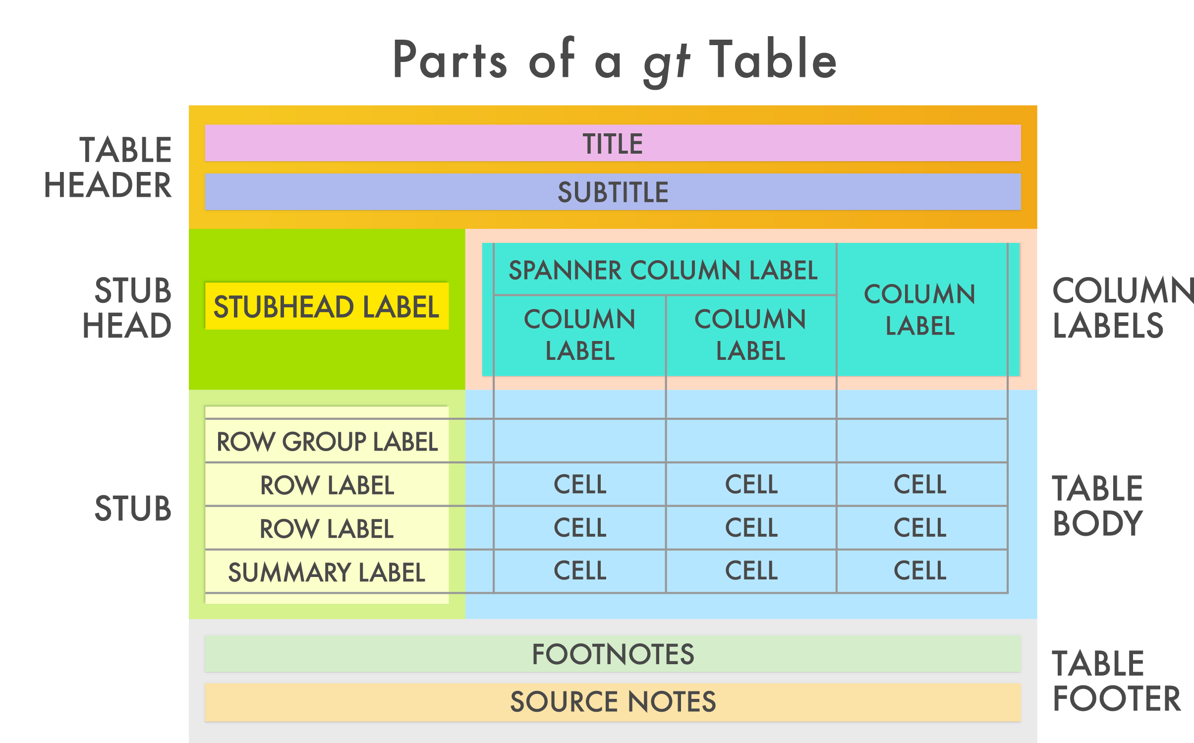
Just as we build our plots in ggplot2 with layers, we can build gt tables by editing each part or layer of the table. As the gt developers outline: “The gt philosophy: we can construct a wide variety of useful tables with a cohesive set of table parts. These include the table header, the stub, the column labels and spanner column labels, the table body, and the table footer.”

The gt package webpages have an excellent introduction to greating gt Tables, which you can find here.

Thomas Mock has some excellent resources on his blog as well which you may find helpful in getting accustomed to the gt package and its wide-ranging functionalities: gt cookbook as well as the advanced gt cookbook and more advanced making beautiful tables with gtExtra.

Note: You are not expected to master gt nor the advanced elements of gt for this course. If you are interested, some advanced resources are included here. The gt introduction and gt cookbook would are a good place to start if you wish to explore the package and creating tables over and above what is covered in this optional Topic.

The gt table workflow

Not only is gt like ggplot2 but for tables, but it also follows tidyverse conventions! This means you can pipe your wrangled data into the gt() function seemlessly.

A typical gt Table workflow is visualized below:

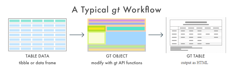
You begin with a preprocessed tabular data, such as a tibble. Next you create your gt table and customize it to your needs. Finally, the table is rendered by printing it at the console, including it in an R Markdown document, or exporting to a file using the gtsave() function.

The code can look a bit scary, but do not fear! Think about it as writing down in code all of the edits that you would make to a table in Word - only now it is reproducible as you have written this in code!

An example of gt workflow

The data

As with everything we have learned about in programming in this course, we must first start with the data.

We will be using a new dataset from Public Health Scotland:

Stroke Mortality by Health Board

Let’s start out with some data wrangling to get the data ready for presentation in a table

# load libraries 
 library(tidyverse)  
 library(gt) # remember to install gt in the first instance with install.packages("gt")
 
 # import data
 stroke_mortality_raw <- read_csv("https://www.opendata.nhs.scot/dataset/f5dcf382-e6ca-49f6-b807-4f9cc29555bc/resource/19c01b59-6cf7-42a9-876a-b07b9b92d6eb/download/stroke_mortalitybyhbr.csv")
 
 hb <- read_csv("https://www.opendata.nhs.scot/dataset/9f942fdb-e59e-44f5-b534-d6e17229cc7b/resource/652ff726-e676-4a20-abda-435b98dd7bdc/download/hb14_hb19.csv")
 
 stroke_mortality <- stroke_mortality_raw %>%
 # Join cancelled to hb
   left_join(hb, join_by(Hbr == HB)) %>%
 # select the variables we are interested in 
   select(Year, HBName, AgeGroup, Sex, Diagnosis, NumberOfDeaths, CrudeRate, EASR) %>% 
 # filter out aggregate levels of the variables 
   filter(Sex != "All" & AgeGroup != "All")

Create a gt table with `gt()`

For sake of simplicity, let’s say that we are specifically interested in the year 2020, adults 75 years old or older, and in 2 Health Boards: NHS Borders and NHS Fife.

To create a gt table object, all you need to do is pass your dataset, plus any data wrangling, to the gt() function. Because the gt package follows tidyverse conventions, our good friend the pipe (%>%) will continue to be useful to us here to use the gt functions to modify the gt table object!

stroke_mortality %>%
   filter(Year == 2020,
          AgeGroup == "75plus years",
          HBName %in% c("NHS Borders", "NHS Fife")) %>% 
   gt()

Year	HBName	AgeGroup	Sex	Diagnosis	NumberOfDeaths	CrudeRate	EASR
2020	NHS Borders	75plus years	Male	Cerebrovascular Disease	23	393.633407	424.306091
2020	NHS Borders	75plus years	Female	Cerebrovascular Disease	46	617.947340	609.187745
2020	NHS Fife	75plus years	Male	Cerebrovascular Disease	98	667.393081	757.712097
2020	NHS Fife	75plus years	Female	Cerebrovascular Disease	151	761.818274	742.539160
2020	NHS Borders	75plus years	Male	stroke	17	290.946432	314.000526
2020	NHS Borders	75plus years	Female	stroke	35	470.177324	463.058843
2020	NHS Fife	75plus years	Male	stroke	52	354.126941	396.146064
2020	NHS Fife	75plus years	Female	stroke	87	438.928409	428.374773
2020	NHS Borders	75plus years	Male	Subaracahnoid Haemorrhage	1	17.114496	16.835017
2020	NHS Borders	75plus years	Female	Subaracahnoid Haemorrhage	1	13.433638	14.804945
2020	NHS Fife	75plus years	Male	Subaracahnoid Haemorrhage	1	6.810133	10.797970
2020	NHS Fife	75plus years	Female	Subaracahnoid Haemorrhage	1	5.045154	5.460676
2020	NHS Borders	75plus years	Male	TIAs and related syndromes	0	0.000000	0.000000
2020	NHS Borders	75plus years	Female	TIAs and related syndromes	0	0.000000	0.000000
2020	NHS Fife	75plus years	Male	TIAs and related syndromes	0	0.000000	0.000000
2020	NHS Fife	75plus years	Female	TIAs and related syndromes	1	5.045154	5.059705

Because we have filtered the data to only be for one Year and one AgeGroup, it is not necessarily relevant to include them in the table as we can highlight what data is presented in the table title (covered later in this tutorial). In this case, you can first select only the variables you are interested in showing in the table before creating the gt object.

stroke_mortality %>%
   filter(Year == 2020,
          AgeGroup == "75plus years",
          HBName %in% c("NHS Borders", "NHS Fife")) %>% 
   select(HBName, 
          Sex, 
          Diagnosis, 
          NumberOfDeaths, 
          CrudeRate, 
          EASR) %>% 
   gt()

HBName	Sex	Diagnosis	NumberOfDeaths	CrudeRate	EASR
NHS Borders	Male	Cerebrovascular Disease	23	393.633407	424.306091
NHS Borders	Female	Cerebrovascular Disease	46	617.947340	609.187745
NHS Fife	Male	Cerebrovascular Disease	98	667.393081	757.712097
NHS Fife	Female	Cerebrovascular Disease	151	761.818274	742.539160
NHS Borders	Male	stroke	17	290.946432	314.000526
NHS Borders	Female	stroke	35	470.177324	463.058843
NHS Fife	Male	stroke	52	354.126941	396.146064
NHS Fife	Female	stroke	87	438.928409	428.374773
NHS Borders	Male	Subaracahnoid Haemorrhage	1	17.114496	16.835017
NHS Borders	Female	Subaracahnoid Haemorrhage	1	13.433638	14.804945
NHS Fife	Male	Subaracahnoid Haemorrhage	1	6.810133	10.797970
NHS Fife	Female	Subaracahnoid Haemorrhage	1	5.045154	5.460676
NHS Borders	Male	TIAs and related syndromes	0	0.000000	0.000000
NHS Borders	Female	TIAs and related syndromes	0	0.000000	0.000000
NHS Fife	Male	TIAs and related syndromes	0	0.000000	0.000000
NHS Fife	Female	TIAs and related syndromes	1	5.045154	5.059705

Modify columns with the cols_*() functions

Column labels, cell alignment, column width, and placement as well as combine multiple columns with the range of cols_*() functions.

For example, cols_label() is particularly useful to rename columns to more informative names than what the variable is called in the dataset. This changes the labels of the columns, as per the function name, not the underlying column names (which remain the name of the variable in your dataset). Tables should be able to be understood by people who are not familiar with your dataset, so it is important for your variables to have informative names.

stroke_mortality %>%
   filter(Year == 2020,
          AgeGroup == "75plus years",
          HBName %in% c("NHS Borders", "NHS Fife")) %>% 
   select(HBName, 
          Sex, 
          Diagnosis, 
          NumberOfDeaths, 
          CrudeRate, 
          EASR) %>% 
   gt() %>% 
   cols_label(HBName = "Health Board",
              NumberOfDeaths = "Number of Deaths",
              CrudeRate = "Crude Rate", 
              EASR = "European Age-Sex Standardised Rate")

Health Board	Sex	Diagnosis	Number of Deaths	Crude Rate	European Age-Sex Standardised Rate
NHS Borders	Male	Cerebrovascular Disease	23	393.633407	424.306091
NHS Borders	Female	Cerebrovascular Disease	46	617.947340	609.187745
NHS Fife	Male	Cerebrovascular Disease	98	667.393081	757.712097
NHS Fife	Female	Cerebrovascular Disease	151	761.818274	742.539160
NHS Borders	Male	stroke	17	290.946432	314.000526
NHS Borders	Female	stroke	35	470.177324	463.058843
NHS Fife	Male	stroke	52	354.126941	396.146064
NHS Fife	Female	stroke	87	438.928409	428.374773
NHS Borders	Male	Subaracahnoid Haemorrhage	1	17.114496	16.835017
NHS Borders	Female	Subaracahnoid Haemorrhage	1	13.433638	14.804945
NHS Fife	Male	Subaracahnoid Haemorrhage	1	6.810133	10.797970
NHS Fife	Female	Subaracahnoid Haemorrhage	1	5.045154	5.460676
NHS Borders	Male	TIAs and related syndromes	0	0.000000	0.000000
NHS Borders	Female	TIAs and related syndromes	0	0.000000	0.000000
NHS Fife	Male	TIAs and related syndromes	0	0.000000	0.000000
NHS Fife	Female	TIAs and related syndromes	1	5.045154	5.059705

cols_align() aligns all text within a column. You can specify which columns to align using vars() - notice that the arguments are the original variable names. Commonly, the convention is to left-align text with varying length and right-align numbers. You can align different columns different ways by adding multiple cols_align() layers.

stroke_mortality %>%
   filter(Year == 2020,
          AgeGroup == "75plus years",
          HBName %in% c("NHS Borders", "NHS Fife")) %>% 
   select(HBName, 
          Sex, 
          Diagnosis,
          NumberOfDeaths,
          CrudeRate, 
          EASR) %>% 
   gt() %>% 
   cols_label(HBName = "Health Board",
              NumberOfDeaths = "Number of Deaths",
              CrudeRate = "Crude Rate", 
              EASR = "European Age-Sex Standardised Rate") %>% 
   cols_align(align = "center",
              columns = NumberOfDeaths)

Health Board	Sex	Diagnosis	Number of Deaths	Crude Rate	European Age-Sex Standardised Rate
NHS Borders	Male	Cerebrovascular Disease	23	393.633407	424.306091
NHS Borders	Female	Cerebrovascular Disease	46	617.947340	609.187745
NHS Fife	Male	Cerebrovascular Disease	98	667.393081	757.712097
NHS Fife	Female	Cerebrovascular Disease	151	761.818274	742.539160
NHS Borders	Male	stroke	17	290.946432	314.000526
NHS Borders	Female	stroke	35	470.177324	463.058843
NHS Fife	Male	stroke	52	354.126941	396.146064
NHS Fife	Female	stroke	87	438.928409	428.374773
NHS Borders	Male	Subaracahnoid Haemorrhage	1	17.114496	16.835017
NHS Borders	Female	Subaracahnoid Haemorrhage	1	13.433638	14.804945
NHS Fife	Male	Subaracahnoid Haemorrhage	1	6.810133	10.797970
NHS Fife	Female	Subaracahnoid Haemorrhage	1	5.045154	5.460676
NHS Borders	Male	TIAs and related syndromes	0	0.000000	0.000000
NHS Borders	Female	TIAs and related syndromes	0	0.000000	0.000000
NHS Fife	Male	TIAs and related syndromes	0	0.000000	0.000000
NHS Fife	Female	TIAs and related syndromes	1	5.045154	5.059705

cols_move_*() set of functions allows you to move columns to the start or end (or wherever you want!) in your table. To move a column to the start we use cols_move_to_start() and to move a column to the end, the function is cols_move_to_end().

stroke_mortality %>%
  filter(Year == 2020,
         AgeGroup == "75plus years",
         HBName %in% c("NHS Borders", "NHS Fife")) %>% 
  select(HBName, 
         Sex, 
         Diagnosis, 
         NumberOfDeaths, 
         CrudeRate, 
         EASR) %>% 
  gt() %>% 
# to move the diagnosis and Sex columns to the start 
  cols_move_to_start(columns = c(Diagnosis, Sex)) %>% 
# to move the HBName after Number of Deaths 
  cols_move(columns = HBName, after = NumberOfDeaths) %>% 
  cols_label(HBName = "Health Board",
             NumberOfDeaths = "Number of Deaths",
             CrudeRate = "Crude Rate", 
             EASR = "European Age-Sex Standardised Rate") %>% 
 cols_align(align = "center", columns = NumberOfDeaths)

Diagnosis	Sex	Number of Deaths	Health Board	Crude Rate	European Age-Sex Standardised Rate
Cerebrovascular Disease	Male	23	NHS Borders	393.633407	424.306091
Cerebrovascular Disease	Female	46	NHS Borders	617.947340	609.187745
Cerebrovascular Disease	Male	98	NHS Fife	667.393081	757.712097
Cerebrovascular Disease	Female	151	NHS Fife	761.818274	742.539160
stroke	Male	17	NHS Borders	290.946432	314.000526
stroke	Female	35	NHS Borders	470.177324	463.058843
stroke	Male	52	NHS Fife	354.126941	396.146064
stroke	Female	87	NHS Fife	438.928409	428.374773
Subaracahnoid Haemorrhage	Male	1	NHS Borders	17.114496	16.835017
Subaracahnoid Haemorrhage	Female	1	NHS Borders	13.433638	14.804945
Subaracahnoid Haemorrhage	Male	1	NHS Fife	6.810133	10.797970
Subaracahnoid Haemorrhage	Female	1	NHS Fife	5.045154	5.460676
TIAs and related syndromes	Male	0	NHS Borders	0.000000	0.000000
TIAs and related syndromes	Female	0	NHS Borders	0.000000	0.000000
TIAs and related syndromes	Male	0	NHS Fife	0.000000	0.000000
TIAs and related syndromes	Female	1	NHS Fife	5.045154	5.059705

Format columns with the fmt_*() functions

To format values within columns, you can use the range of fmt_*() functions.

fmt_number() formats numeric (number-based) columns. For example, using the argument decimal = 2 you can set a decimal place or add a suffix such as K for thousands to large numbers using suffixing = TRUE.

stroke_mortality %>%
   filter(Year == 2020,
          AgeGroup == "75plus years",
          HBName %in% c("NHS Borders", "NHS Fife")) %>% 
   select(HBName, Sex, Diagnosis, NumberOfDeaths, CrudeRate, EASR) %>% 
   gt() %>%
   fmt_number(columns = c(CrudeRate, EASR), decimals = 3)

HBName	Sex	Diagnosis	NumberOfDeaths	CrudeRate	EASR
NHS Borders	Male	Cerebrovascular Disease	23	393.633	424.306
NHS Borders	Female	Cerebrovascular Disease	46	617.947	609.188
NHS Fife	Male	Cerebrovascular Disease	98	667.393	757.712
NHS Fife	Female	Cerebrovascular Disease	151	761.818	742.539
NHS Borders	Male	stroke	17	290.946	314.001
NHS Borders	Female	stroke	35	470.177	463.059
NHS Fife	Male	stroke	52	354.127	396.146
NHS Fife	Female	stroke	87	438.928	428.375
NHS Borders	Male	Subaracahnoid Haemorrhage	1	17.114	16.835
NHS Borders	Female	Subaracahnoid Haemorrhage	1	13.434	14.805
NHS Fife	Male	Subaracahnoid Haemorrhage	1	6.810	10.798
NHS Fife	Female	Subaracahnoid Haemorrhage	1	5.045	5.461
NHS Borders	Male	TIAs and related syndromes	0	0.000	0.000
NHS Borders	Female	TIAs and related syndromes	0	0.000	0.000
NHS Fife	Male	TIAs and related syndromes	0	0.000	0.000
NHS Fife	Female	TIAs and related syndromes	1	5.045	5.060

fmt_percent() formats numbers into percents and includes the % symbol for us. By default, the values are multiplied by 100 before adding the % symbol. So, if your data is already multiplied by 100, use the scale_value = FALSE argument to tell R that the input is not a proportion.

stroke_mortality %>%
  filter(Year == 2020,
          AgeGroup == "75plus years",
          HBName %in% c("NHS Borders", "NHS Fife")) %>% 
  select(HBName,
         Sex, 
         Diagnosis,
         NumberOfDeaths, 
         CrudeRate, 
         EASR) %>%
  gt() %>%
  fmt_percent(columns = c(CrudeRate, EASR), decimals = 0, scale_value = FALSE)

HBName	Sex	Diagnosis	NumberOfDeaths	CrudeRate	EASR
NHS Borders	Male	Cerebrovascular Disease	23	394%	424%
NHS Borders	Female	Cerebrovascular Disease	46	618%	609%
NHS Fife	Male	Cerebrovascular Disease	98	667%	758%
NHS Fife	Female	Cerebrovascular Disease	151	762%	743%
NHS Borders	Male	stroke	17	291%	314%
NHS Borders	Female	stroke	35	470%	463%
NHS Fife	Male	stroke	52	354%	396%
NHS Fife	Female	stroke	87	439%	428%
NHS Borders	Male	Subaracahnoid Haemorrhage	1	17%	17%
NHS Borders	Female	Subaracahnoid Haemorrhage	1	13%	15%
NHS Fife	Male	Subaracahnoid Haemorrhage	1	7%	11%
NHS Fife	Female	Subaracahnoid Haemorrhage	1	5%	5%
NHS Borders	Male	TIAs and related syndromes	0	0%	0%
NHS Borders	Female	TIAs and related syndromes	0	0%	0%
NHS Fife	Male	TIAs and related syndromes	0	0%	0%
NHS Fife	Female	TIAs and related syndromes	1	5%	5%

sub_missing() formats the default NA missing values in R to be a dash instead. As the subset of data we have been using does not have any NAs, we need to first change the data filtering a bit of our code to include NA values.

stroke_mortality %>% 
  filter(Year == 2012,
         AgeGroup == "75plus years",
         HBName %in% c("NHS Orkney", "NHS Grampian")) %>% 
  select(-Year, -AgeGroup) %>%
  gt() %>%
  sub_missing(columns = c(NumberOfDeaths, CrudeRate))

HBName	Sex	Diagnosis	NumberOfDeaths	CrudeRate	EASR

…and now to the stub (or rows)!

The stub is typically a column of row labels that does not have or need a column label.

Add a grouping using the `rowname_col` argument

There are two ways in which you can add a grouping variable to your table, which differ in aesthetics

by passing grouped data to the gt() function

 stroke_mortality %>%
  filter(Year == 2020,
         AgeGroup == "75plus years",
         HBName %in% c("NHS Borders", "NHS Fife")) %>% 
  select(-Year, - AgeGroup) %>%
  group_by(Sex) %>%
  gt()

HBName	Diagnosis	NumberOfDeaths	CrudeRate	EASR
Male
NHS Borders	Cerebrovascular Disease	23	393.633407	424.306091
NHS Fife	Cerebrovascular Disease	98	667.393081	757.712097
NHS Borders	stroke	17	290.946432	314.000526
NHS Fife	stroke	52	354.126941	396.146064
NHS Borders	Subaracahnoid Haemorrhage	1	17.114496	16.835017
NHS Fife	Subaracahnoid Haemorrhage	1	6.810133	10.797970
NHS Borders	TIAs and related syndromes	0	0.000000	0.000000
NHS Fife	TIAs and related syndromes	0	0.000000	0.000000
Female
NHS Borders	Cerebrovascular Disease	46	617.947340	609.187745
NHS Fife	Cerebrovascular Disease	151	761.818274	742.539160
NHS Borders	stroke	35	470.177324	463.058843
NHS Fife	stroke	87	438.928409	428.374773
NHS Borders	Subaracahnoid Haemorrhage	1	13.433638	14.804945
NHS Fife	Subaracahnoid Haemorrhage	1	5.045154	5.460676
NHS Borders	TIAs and related syndromes	0	0.000000	0.000000
NHS Fife	TIAs and related syndromes	1	5.045154	5.059705

specify rowname_col within gt()

stroke_mortality %>%
  filter(Year == 2020,
         AgeGroup == "75plus years",
         HBName %in% c("NHS Borders", "NHS Fife")) %>% 
  select(-Year, - AgeGroup) %>%
  gt(rowname_col = "Sex")

	HBName	Diagnosis	NumberOfDeaths	CrudeRate	EASR
Male	NHS Borders	Cerebrovascular Disease	23	393.633407	424.306091
Female	NHS Borders	Cerebrovascular Disease	46	617.947340	609.187745
Male	NHS Fife	Cerebrovascular Disease	98	667.393081	757.712097
Female	NHS Fife	Cerebrovascular Disease	151	761.818274	742.539160
Male	NHS Borders	stroke	17	290.946432	314.000526
Female	NHS Borders	stroke	35	470.177324	463.058843
Male	NHS Fife	stroke	52	354.126941	396.146064
Female	NHS Fife	stroke	87	438.928409	428.374773
Male	NHS Borders	Subaracahnoid Haemorrhage	1	17.114496	16.835017
Female	NHS Borders	Subaracahnoid Haemorrhage	1	13.433638	14.804945
Male	NHS Fife	Subaracahnoid Haemorrhage	1	6.810133	10.797970
Female	NHS Fife	Subaracahnoid Haemorrhage	1	5.045154	5.460676
Male	NHS Borders	TIAs and related syndromes	0	0.000000	0.000000
Female	NHS Borders	TIAs and related syndromes	0	0.000000	0.000000
Male	NHS Fife	TIAs and related syndromes	0	0.000000	0.000000
Female	NHS Fife	TIAs and related syndromes	1	5.045154	5.059705

To add a column name to the stub, if desired, you can use tab_stubhead().

stroke_mortality %>%
  filter(Year == 2020,
         AgeGroup == "75plus years",
         HBName %in% c("NHS Borders", "NHS Fife")) %>% 
  #select(-Year, - AgeGroup) %>%
  group_by(Sex) %>% 
  gt() %>% 
  summary_rows(columns = NumberOfDeaths, 
               fns = list("Average" = ~mean(., na.rm = TRUE)))

	Year	HBName	AgeGroup	Diagnosis	NumberOfDeaths	CrudeRate	EASR
Male
	2020	NHS Borders	75plus years	Cerebrovascular Disease	23	393.633407	424.306091
	2020	NHS Fife	75plus years	Cerebrovascular Disease	98	667.393081	757.712097
	2020	NHS Borders	75plus years	stroke	17	290.946432	314.000526
	2020	NHS Fife	75plus years	stroke	52	354.126941	396.146064
	2020	NHS Borders	75plus years	Subaracahnoid Haemorrhage	1	17.114496	16.835017
	2020	NHS Fife	75plus years	Subaracahnoid Haemorrhage	1	6.810133	10.797970
	2020	NHS Borders	75plus years	TIAs and related syndromes	0	0.000000	0.000000
	2020	NHS Fife	75plus years	TIAs and related syndromes	0	0.000000	0.000000
Average	—	—	—	—	24.00	—	—
Female
	2020	NHS Borders	75plus years	Cerebrovascular Disease	46	617.947340	609.187745
	2020	NHS Fife	75plus years	Cerebrovascular Disease	151	761.818274	742.539160
	2020	NHS Borders	75plus years	stroke	35	470.177324	463.058843
	2020	NHS Fife	75plus years	stroke	87	438.928409	428.374773
	2020	NHS Borders	75plus years	Subaracahnoid Haemorrhage	1	13.433638	14.804945
	2020	NHS Fife	75plus years	Subaracahnoid Haemorrhage	1	5.045154	5.460676
	2020	NHS Borders	75plus years	TIAs and related syndromes	0	0.000000	0.000000
	2020	NHS Fife	75plus years	TIAs and related syndromes	1	5.045154	5.059705
Average	—	—	—	—	40.25	—	—

You can also add grand summaries to grouped data using grand_summary_rows().

stroke_mortality %>%
  filter(Year == 2020,
         AgeGroup == "75plus years",
         HBName %in% c("NHS Borders", "NHS Fife")) %>% 
  select(-Year, - AgeGroup) %>%   
  group_by(Sex) %>% 
  gt() %>% 
  summary_rows(columns = c(NumberOfDeaths, CrudeRate, EASR), 
               fns = list(Average = ~mean(., na.rm = TRUE))) %>% 
  grand_summary_rows(columns = c(NumberOfDeaths, CrudeRate, EASR), 
                     fns = list("Overall Average" = ~mean(., na.rm = TRUE)))

	HBName	Diagnosis	NumberOfDeaths	CrudeRate	EASR
Male
	NHS Borders	Cerebrovascular Disease	23	393.633407	424.306091
	NHS Fife	Cerebrovascular Disease	98	667.393081	757.712097
	NHS Borders	stroke	17	290.946432	314.000526
	NHS Fife	stroke	52	354.126941	396.146064
	NHS Borders	Subaracahnoid Haemorrhage	1	17.114496	16.835017
	NHS Fife	Subaracahnoid Haemorrhage	1	6.810133	10.797970
	NHS Borders	TIAs and related syndromes	0	0.000000	0.000000
	NHS Fife	TIAs and related syndromes	0	0.000000	0.000000
Average	—	—	24.00	216.2531	239.9747
Female
	NHS Borders	Cerebrovascular Disease	46	617.947340	609.187745
	NHS Fife	Cerebrovascular Disease	151	761.818274	742.539160
	NHS Borders	stroke	35	470.177324	463.058843
	NHS Fife	stroke	87	438.928409	428.374773
	NHS Borders	Subaracahnoid Haemorrhage	1	13.433638	14.804945
	NHS Fife	Subaracahnoid Haemorrhage	1	5.045154	5.460676
	NHS Borders	TIAs and related syndromes	0	0.000000	0.000000
	NHS Fife	TIAs and related syndromes	1	5.045154	5.059705
Average	—	—	40.25	289.0494	283.5607
Overall Average	—	—	32.125	252.6512	261.7677

You may have noticed that the decimal places are all of the place in the above table. It is good practice to have a consistent reporting of numbers to the same decimal place. We can sort out the columns with fmt_number() which have have seen previously and the summary rows with the argument fmt.

stroke_mortality %>%
  filter(Year == 2020,
         AgeGroup == "75plus years",
         HBName %in% c("NHS Borders", "NHS Fife")) %>% 
  select(-Year, - AgeGroup) %>%   
  group_by(Sex) %>% 
  gt() %>% 
  # format numbers in columns 
  fmt_number(columns = c(CrudeRate, EASR), decimals = 3) %>% 
  summary_rows(columns = c(NumberOfDeaths, CrudeRate, EASR), 
               fns = list(Average = ~mean(., na.rm = TRUE)),
               # format number in grouped summary rows 
               fmt = list(~ fmt_number(., decimals = 3))) %>% 
  grand_summary_rows(columns = c(NumberOfDeaths, CrudeRate, EASR), 
                     fns = list("Overall Average" = ~mean(., na.rm = TRUE)),
                     # and format number in grand summary row 
                     fmt = list(~ fmt_number(., decimals = 3)))

	HBName	Diagnosis	NumberOfDeaths	CrudeRate	EASR
Male
	NHS Borders	Cerebrovascular Disease	23	393.633	424.306
	NHS Fife	Cerebrovascular Disease	98	667.393	757.712
	NHS Borders	stroke	17	290.946	314.001
	NHS Fife	stroke	52	354.127	396.146
	NHS Borders	Subaracahnoid Haemorrhage	1	17.114	16.835
	NHS Fife	Subaracahnoid Haemorrhage	1	6.810	10.798
	NHS Borders	TIAs and related syndromes	0	0.000	0.000
	NHS Fife	TIAs and related syndromes	0	0.000	0.000
Average	—	—	24.000	216.253	239.975
Female
	NHS Borders	Cerebrovascular Disease	46	617.947	609.188
	NHS Fife	Cerebrovascular Disease	151	761.818	742.539
	NHS Borders	stroke	35	470.177	463.059
	NHS Fife	stroke	87	438.928	428.375
	NHS Borders	Subaracahnoid Haemorrhage	1	13.434	14.805
	NHS Fife	Subaracahnoid Haemorrhage	1	5.045	5.461
	NHS Borders	TIAs and related syndromes	0	0.000	0.000
	NHS Fife	TIAs and related syndromes	1	5.045	5.060
Average	—	—	40.250	289.049	283.561
Overall Average	—	—	32.125	252.651	261.768

Add the final touches

Once you have your table formatted as you would like, it is important to add the final touches to make it formative for your target audience, including a header (title) and any notes.

Add a title and/or subtitle using tab_header().

stroke_mortality %>%
  filter(Year == 2020,
         AgeGroup == "75plus years",
         HBName %in% c("NHS Borders", "NHS Fife")) %>% 
  select(-Year, - AgeGroup) %>%   
  gt() %>% 
  tab_header(title = "Stroke Mortality in 2020 in Adults Aged 75+",
             subtitle = "Data from NHS Borders and NHS Fife")

HBName	Sex	Diagnosis	NumberOfDeaths	CrudeRate	EASR
Stroke Mortality in 2020 in Adults Aged 75+
Data from NHS Borders and NHS Fife
NHS Borders	Male	Cerebrovascular Disease	23	393.633407	424.306091
NHS Borders	Female	Cerebrovascular Disease	46	617.947340	609.187745
NHS Fife	Male	Cerebrovascular Disease	98	667.393081	757.712097
NHS Fife	Female	Cerebrovascular Disease	151	761.818274	742.539160
NHS Borders	Male	stroke	17	290.946432	314.000526
NHS Borders	Female	stroke	35	470.177324	463.058843
NHS Fife	Male	stroke	52	354.126941	396.146064
NHS Fife	Female	stroke	87	438.928409	428.374773
NHS Borders	Male	Subaracahnoid Haemorrhage	1	17.114496	16.835017
NHS Borders	Female	Subaracahnoid Haemorrhage	1	13.433638	14.804945
NHS Fife	Male	Subaracahnoid Haemorrhage	1	6.810133	10.797970
NHS Fife	Female	Subaracahnoid Haemorrhage	1	5.045154	5.460676
NHS Borders	Male	TIAs and related syndromes	0	0.000000	0.000000
NHS Borders	Female	TIAs and related syndromes	0	0.000000	0.000000
NHS Fife	Male	TIAs and related syndromes	0	0.000000	0.000000
NHS Fife	Female	TIAs and related syndromes	1	5.045154	5.059705

You can also add spanner column labels if you have multiple similar variables and would like to draw attention to the grouping using tab_spanner(). You can use multiple tab_spanner() layers to add multiple spanners highlighting different groups of columns.

stroke_mortality %>%
  filter(Year == 2020,
         AgeGroup == "75plus years",
         HBName %in% c("NHS Borders", "NHS Fife")) %>% 
  select(-Year, - AgeGroup) %>%  
  gt() %>%
  tab_header(title = "Stroke Mortality in 2020 in Adults Aged 75+",
             subtitle = "Data from NHS Borders and NHS Fife") %>% 
  tab_spanner(label = "Rate per 100k population",
              columns = c(CrudeRate, EASR))

HBName	Sex	Diagnosis	NumberOfDeaths	Rate per 100k population
Stroke Mortality in 2020 in Adults Aged 75+
Data from NHS Borders and NHS Fife
HBName	Sex	Diagnosis	NumberOfDeaths	CrudeRate	EASR
NHS Borders	Male	Cerebrovascular Disease	23	393.633407	424.306091
NHS Borders	Female	Cerebrovascular Disease	46	617.947340	609.187745
NHS Fife	Male	Cerebrovascular Disease	98	667.393081	757.712097
NHS Fife	Female	Cerebrovascular Disease	151	761.818274	742.539160
NHS Borders	Male	stroke	17	290.946432	314.000526
NHS Borders	Female	stroke	35	470.177324	463.058843
NHS Fife	Male	stroke	52	354.126941	396.146064
NHS Fife	Female	stroke	87	438.928409	428.374773
NHS Borders	Male	Subaracahnoid Haemorrhage	1	17.114496	16.835017
NHS Borders	Female	Subaracahnoid Haemorrhage	1	13.433638	14.804945
NHS Fife	Male	Subaracahnoid Haemorrhage	1	6.810133	10.797970
NHS Fife	Female	Subaracahnoid Haemorrhage	1	5.045154	5.460676
NHS Borders	Male	TIAs and related syndromes	0	0.000000	0.000000
NHS Borders	Female	TIAs and related syndromes	0	0.000000	0.000000
NHS Fife	Male	TIAs and related syndromes	0	0.000000	0.000000
NHS Fife	Female	TIAs and related syndromes	1	5.045154	5.059705

Bonus - Introduction video from `gt` package developers

Rich Iannone is one of the developers of the gt package. You can watch this video where he introduces the package and does a live walk through of creating gt tables.