library(tidyverse)

# create a new tibble called x
x <- tibble(id = c(1, 2, 3, 4, 5),
            x = c("x1", "x2", "x3", "x4", "x5"))
print(x)Topic 1: Wrangling factors and joins
Working with Factors
Factors were mentioned very briefly in Week 2 of this course.
Let’s just recap. Here is how we described them:
Factors can be thought of as slightly fussy characters. They’re fussy because they have something called levels. Levels are all the unique values this variable could take e.g. if we have a column with data on sex, there might be two levels, “Male” and “Female” or there might be three levels if there was an option to specify “Other” too. Using factors rather than just characters can be useful because:
The values that factor levels can take is fixed. For example, if the predefined levels of your column called sex are “Male” and “Female” and you try to add a new patient where sex is just called “F” you will get a warning from R. If the column sex was stored as a character data type rather than a factor, R would have no problem with this and you would end up with “Male”, “Female”, and “F” in your column.
Levels have an order. By default R sorts things alphabetically, but if you want to use a non-alphabetical order, e.g. if we had a body_weight variable where we want the levels to be ordered - “underweight”-“normal weight”-“overweight” - we need make body_weight into a factor. Making a character column into a factor enables us to define and change the order of the levels.
These can be huge benefits, especially as a lot of medical data analyses include the comparison of different risks to a reference level. There is a handy cheatsheet around the forcats package in R, which provides tools for working with factor (or categorical data).
Factors Practice
Remember to begin by creating a new project in RStudio.
Then download the R Markdown document and associated CSV files by right clicking on the links below and choosing, Save Link As. Then navigate to your newly created project folder, and save.
Note: There is some optional, advanced Bonus Content at the end of this practice document.
Have fun!
Often the data you want to work with is spread between multiple tables or spreadsheets. Before you can begin analysing it, you need to know how to combine these datasets. There are a number of different ways you can join your data together, although you’ll probably find yourself using just a couple of these joins on a regular basis.
The ones we’ll cover here are:
left_join()inner_join()full_join()
When joining two sets of data, R will look for a common column or columns on which to join. If it finds a name and data type match then it will join on this/these unless told otherwise.
For demonstration purposes, the code below creates two tibbles (tidyverse data frames), x and y with a column in common, id , which we can imagine is patient id. Let’s also imagine that the two tibbles created here contain different information about a group of patients: x might be about outpatient appointments and y about treatments. You will see that we have intentionally included some patients in both tibbles but there are some only in tibble x and some only in tibble y. We now want to combine these tibbles for analysis.
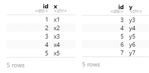
# create a new tibble called y
y <- tibble(id = c(3, 4, 5, 6, 7),
            y = c("y3", "y4", "y5", "y6", "y7"))
y
Which join you choose depends on which rows you want to keep and from which datasets. In the joins we’ll be discussing below, all columns from both datasets are kept.
I want to keep all data from both x and y
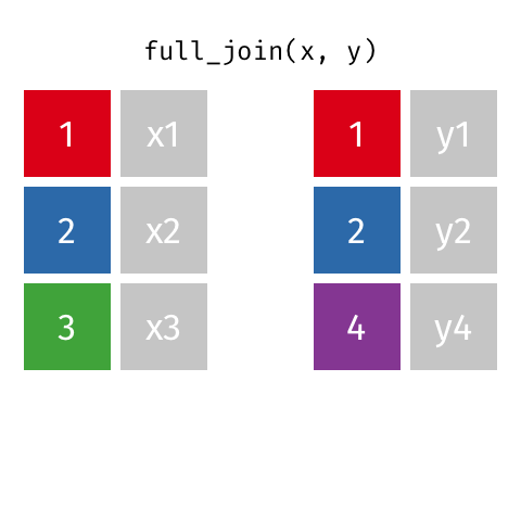
full_join(x, y, by = "id")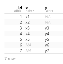
I want to keep all data from x and only matching data from y
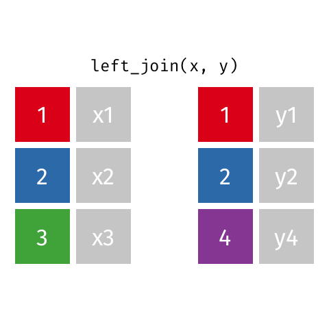
Choose left_join() which keeps all data from the (primary) dataset x and only adds data from (another) dataset y if a match is found with the dataset x. Where no matching value is found for x NA is returned in the y column(s).
left_join(x, y, by = "id")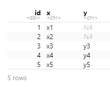
If there is more than one match between x and y (perhaps x is a list of patients and y is a list of medications each patients is on), all combinations of the matches are returned.
I only want to keep data that is matched on both x and y

Choose inner_join() which keeps only rows of data where a match is found between x and y.
inner_join(x, y, by = "id")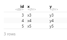
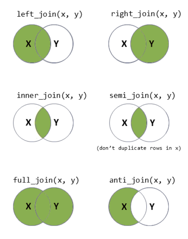
You can also think of joins using Venn diagrams:
To find out more information on the full set of joins you can use, take a look in the Help tab under “join” (or type ?join into the console). The data wrangling with dplyr and tidyr cheatsheet can also be quite helpful.
Saving Wrangled Data, Objects, or Tables
Once you have wrangled your data and/or produced a table or object, you may wish to save and share it with stakeholders or collaborators.
To save a csv file, which can then be opened in Excel or other such software, you can use the write_csv() function, which was discussed in one of the Week 6 Topic 3 practice documents. This function works as follows:
```{r}
write_csv(dataobject, "filename.csv")
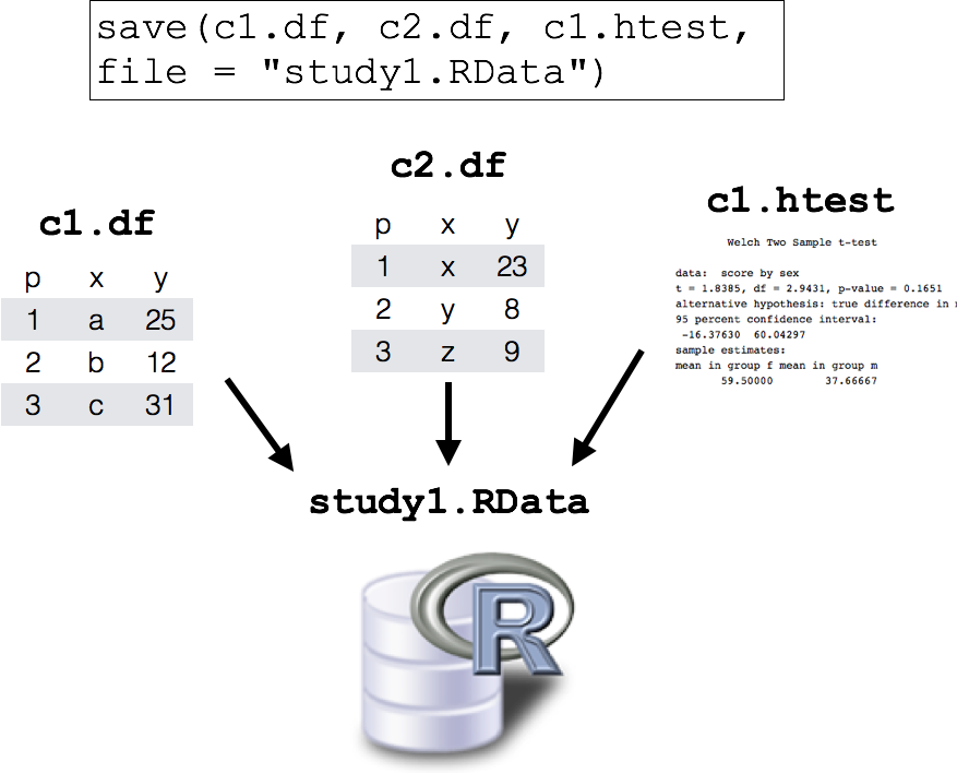
```Alternatively, if you are saving data for your own purposes or to share with a colleague with also uses R, you can create an rda or RData file. rda files are a short form of RData files. The advantages of using RData files include
more quickly restoring data to R for further analysis or wrangling
keeping R specific information encoded in the data (e.g., attributes like factor level order, variable types, etc.)
the option to save multiple objects or tibbles in one file
The functions to save and load RData files are conveniently save() and load(), which work as follows:
```{r}
#to save one object
save(dataobject, "filename.rda")

#to save more than obe object
save(dataobject1, dataobject2, "filename.rda")

#to read in your RData file
load("filename.rda")
```